Measure arrival times in hours after noon, and let Alice’s and Bob’s arrival times be \[ X,Y\sim \operatorname {Unif}(0,1), \] independently.

Since \(X\) and \(Y\) are independent and each has density \[ f_X(x)=f_Y(y)=1, \qquad 0\le x,y\le 1, \] their joint density is \[ f_{X,Y}(x,y) = f_X(x)f_Y(y) = \begin {cases} 1, & 0\le x\le 1,\;0\le y\le 1,\\ 0, & \text {otherwise}. \end {cases} \]

They meet exactly when their arrival times differ by at most 15 minutes, or \(1/4\) of an hour. Thus \[ |X-Y|\le \frac 14. \]

Therefore, \[ \mathbb P\left (|X-Y|\le \frac 14\right ) = \iint _{\{|x-y|\le 1/4\}} f_{X,Y}(x,y)\,dy\,dx. \]

For a fixed \(x\), the condition \[ |x-y|\le \frac 14 \] is equivalent to \[ x-\frac 14\le y\le x+\frac 14. \] Taking into account that \(0\le y\le 1\), we split the integral into three parts: \[ \begin {aligned} \mathbb P\left (|X-Y|\le \frac 14\right ) &= \int _0^{1/4}\int _0^{x+1/4} 1\,dy\,dx\\ &\quad + \int _{1/4}^{3/4}\int _{x-1/4}^{x+1/4} 1\,dy\,dx\\ &\quad + \int _{3/4}^{1}\int _{x-1/4}^{1} 1\,dy\,dx. \end {aligned} \]

Evaluating, \[ \begin {aligned} \mathbb P\left (|X-Y|\le \frac 14\right ) &= \int _0^{1/4}\left (x+\frac 14\right )\,dx + \int _{1/4}^{3/4}\frac 12\,dx + \int _{3/4}^{1}\left (\frac 54-x\right )\,dx\\ &= \frac {3}{32} + \frac 14 + \frac {3}{32}\\ &= \frac {7}{16}. \end {aligned} \]

(a) Since \(X\sim \operatorname {Unif}(0,L)\), we have \[ f_X(x)=\frac 1L,\qquad 0<x<L. \] Given \(X=x\), the random variable \(Y\) is uniform on \((0,x)\), so \[ f_{Y\mid X}(y\mid x)=\frac 1x,\qquad 0<y<x. \] Thus \[ f_{X,Y}(x,y)=f_X(x)f_{Y\mid X}(y\mid x)=\frac {1}{Lx}, \qquad 0<y<x<L. \] It is zero outside this region.

(b) Marginalizing out \(Y\), for \(0<x<L\), gives \[ f_X(x)=\int _0^x \frac {1}{Lx}\,dy=\frac {1}{Lx}\cdot x=\frac 1L. \] This is exactly the \(\operatorname {Unif}(0,L)\) density.

(c) Using the definition of a conditional density, \[ f_{Y\mid X}(y\mid x)=\frac {f_{X,Y}(x,y)}{f_X(x)} =\frac {1/(Lx)}{1/L}=\frac 1x, \qquad 0<y<x. \] This is the uniform density on \((0,x)\), as expected.

(d) For a fixed \(y\), the possible values of \(x\) run from \(y\) to \(L\). Hence, for \(0<y<L\), \[ f_Y(y)=\int _y^L \frac {1}{Lx}\,dx =\frac 1L\log \left (\frac {L}{y}\right ). \]

(e) Finally, \[ f_{X\mid Y}(x\mid y) =\frac {f_{X,Y}(x,y)}{f_Y(y)} =\frac {1/(Lx)}{(1/L)\log (L/y)} =\frac {1}{x\log (L/y)}, \] for \(y<x<L\).

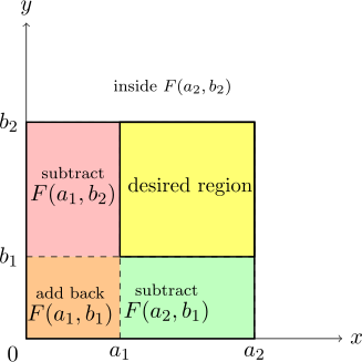
We have covered this fully in the lecture with a visual representation (Lecture 19).

Recall that the joint CDF of \(X\) and \(Y\) is \[ F(x,y)=P(X\le x,\;Y\le y). \]

Since \(X\) and \(Y\) are continuous, let \(f_{X,Y}\) denote their joint density. It is related to the joint CDF by \[ f_{X,Y}(x,y) = \frac {\partial ^2}{\partial x\,\partial y}F(x,y). \]

The probability that \((X,Y)\) falls inside the rectangle \[ [a_1,a_2]\times [b_1,b_2] \] is therefore \[ P(a_1\le X\le a_2,\;b_1\le Y\le b_2) = \int _{a_1}^{a_2}\int _{b_1}^{b_2} f_{X,Y}(x,y)\,dy\,dx. \]

Substituting \[ f_{X,Y}(x,y) = \frac {\partial ^2}{\partial x\,\partial y}F(x,y), \] we obtain \[ \begin {aligned} P(a_1\le X\le a_2,\;b_1\le Y\le b_2) &= \int _{a_1}^{a_2} \int _{b_1}^{b_2} \frac {\partial ^2}{\partial x\,\partial y}F(x,y) \,dy\,dx. \end {aligned} \]

First integrate with respect to \(y\): \[ \begin {aligned} &= \int _{a_1}^{a_2} \left [ \frac {\partial }{\partial x}F(x,y) \right ]_{y=b_1}^{y=b_2} dx\\ &= \int _{a_1}^{a_2} \left ( \frac {\partial }{\partial x}F(x,b_2) - \frac {\partial }{\partial x}F(x,b_1) \right )dx. \end {aligned} \]

Now integrate with respect to \(x\): \[ \begin {aligned} &= \left [F(x,b_2)\right ]_{a_1}^{a_2} - \left [F(x,b_1)\right ]_{a_1}^{a_2}\\ &= \left (F(a_2,b_2)-F(a_1,b_2)\right ) - \left (F(a_2,b_1)-F(a_1,b_1)\right ). \end {aligned} \]

Hence, \[ P(a_1\le X\le a_2,\;b_1\le Y\le b_2) = F(a_2,b_2)-F(a_1,b_2) -F(a_2,b_1)+F(a_1,b_1). \]

Visual reasoning.

Recall that \[ F(a_2,b_2) \] represents all probability mass in the region \[ X\le a_2, \qquad Y\le b_2. \]

Think of this as one large lower-left rectangle extending up to \[ (a_2,b_2). \]

We only want the smaller rectangle \[ a_1\le X\le a_2, \qquad b_1\le Y\le b_2. \]

Starting from \[ {F(a_2,b_2)}, \] we remove the part to the left of \(a_1\): \[ - {F(a_1,b_2)}, \] and remove the part below \(b_1\): \[ - {F(a_2,b_1)}. \]

However, the lower-left corner \[ X\le a_1, \qquad Y\le b_1 \] was contained in both of the pieces we subtracted, so it has been subtracted twice. We therefore add it back once: \[ + {F(a_1,b_1)}. \]

Thus the desired rectangle is obtained by the two-dimensional inclusion–exclusion rule: \[ { \text {desired rectangle} = \text {large rectangle} -\text {left rectangle} -\text {bottom rectangle} +\text {overlap}. } \]

(a) First, note that if \(x,y \in (0,1)\), then \(f_{X,Y}(x,y) = x+y\geq 0\). Otherwise, \(f_{X,Y}(x,y) = 0\geq 0\). So overall, \(f_{X,Y}(x,y)\geq 0 \ \ \forall x,y\in \mathbb {R}\).

Its total integral is \[ \int _0^1\int _0^1 (x+y)\,dy\,dx = \int _0^1\left (x+\frac 12\right )dx =\frac 12+\frac 12=1. \] Thus it is a valid joint PDF.

(b) The variables are not independent. One way to see this is to compute the marginals and observe that their product does not equal the joint density.

(c) For \(0<x<1\), \[ f_X(x)=\int _0^1 (x+y)\,dy=x+\frac 12. \] Similarly, for \(0<y<1\), \[ f_Y(y)=\int _0^1 (x+y)\,dx=y+\frac 12. \]

(d) For \(0<x<1\), the conditional density is \[ f_{Y\mid X}(y\mid x) =\frac {f_{X,Y}(x,y)}{f_X(x)} =\frac {x+y}{x+1/2}, \qquad 0<y<1. \]

(a) We need \[ \int _0^1\int _0^y cxy\,dx\,dy=1. \] The integral is \[ c\int _0^1 y\left (\int _0^y x\,dx\right )dy = c\int _0^1 y\cdot \frac {y^2}{2}\,dy = \frac {c}{2}\cdot \frac 14 = \frac {c}{8}. \] Thus \(c=8\).

(b) The variables are not independent. The support itself already shows this, since the condition \(0<X<Y<1\) ties the possible values of \(X\) and \(Y\) together.

(c) With \(c=8\), for \(0<x<1\), \[ f_X(x)=\int _x^1 8xy\,dy=4x(1-x^2). \] For \(0<y<1\), \[ f_Y(y)=\int _0^y 8xy\,dx=4y^3. \]

(d) For fixed \(x\), the conditional support is \(x<y<1\). Therefore \[ f_{Y\mid X}(y\mid x) =\frac {8xy}{4x(1-x^2)} =\frac {2y}{1-x^2}, \qquad x<y<1. \]

A quadratic polynomial \(Ax^2+Bx+1\) has at least one real root if and only if its discriminant is nonnegative. Therefore, \[ B^2-4A\ge 0. \]

Equivalently, \[ A\le \frac {B^2}{4}. \]

Since \[ A,B\overset {\text {i.i.d.}}{\sim }\operatorname {Unif}(0,1), \] their marginal densities are \[ f_A(a)= \begin {cases} 1, & 0\le a\le 1,\\ 0, & \text {otherwise}, \end {cases} \qquad f_B(b)= \begin {cases} 1, & 0\le b\le 1,\\ 0, & \text {otherwise}. \end {cases} \]

Because \(A\) and \(B\) are independent, their joint density is \[ f_{A,B}(a,b) = f_A(a)f_B(b) = \begin {cases} 1, & 0\le a\le 1,\;0\le b\le 1,\\ 0, & \text {otherwise}. \end {cases} \]

Hence the desired probability is \[ P\left (B^2-4A\ge 0\right ) = P\left (A\le \frac {B^2}{4}\right ). \]

Using the joint density, \[ P\left (A\le \frac {B^2}{4}\right ) = \iint _{\left \{(a,b):\,0\le b\le 1,\, 0\le a\le b^2/4\right \}} f_{A,B}(a,b)\,da\,db. \]

Since \(f_{A,B}(a,b)=1\) on the support, \[ \begin {aligned} P\left (A\le \frac {B^2}{4}\right ) &= \int _0^1 \int _0^{b^2/4} 1\,da\,db\\ &= \int _0^1 \frac {b^2}{4}\,db\\ &= \frac 14 \left [\frac {b^3}{3}\right ]_0^1\\ &= \frac {1}{12} \approx 0.0834 \end {aligned} \] In other words, only 8.34% of such quadratic polynomials have at least one real root!

(a) Since the two dice are independent and identically distributed, \[ \operatorname {Cov}(X+Y,X-Y) = \operatorname {Cov}(X,X)-\operatorname {Cov}(X,Y) +\operatorname {Cov}(Y,X)-\operatorname {Cov}(Y,Y). \] The cross-covariances are zero, and \(\operatorname {Var}(X)=\operatorname {Var}(Y)\). Therefore \[ \operatorname {Cov}(X+Y,X-Y)=\operatorname {Var}(X)-\operatorname {Var}(Y)=0. \] They are not independent. For instance, if \(X+Y=2\), then necessarily \(X=Y=1\), so \(X-Y=0\). Knowing the sum can restrict the difference.

(b) The same covariance calculation applies for independent uniforms. We again get \[ \operatorname {Cov}(X+Y,X-Y)=\operatorname {Var}(X)-\operatorname {Var}(Y)=0. \] They are not independent. The pair \((X+Y,X-Y)\) cannot take arbitrary values in a rectangle. For example, if \(X+Y\) is very close to 0, then both \(X\) and \(Y\) must be close to 0, forcing \(X-Y\) also to be close to 0.

Think of the multinomial vector as coming from \(n\) independent trials, where each trial falls into exactly one of the \(k\) categories. For trial \(r\), define \[ I_{r,i}=\mathbf {1}\{\text {trial }r\text { falls in category }i\}. \] Then \[ X_i=\sum _{r=1}^n I_{r,i}, \qquad X_j=\sum _{s=1}^n I_{s,j}. \] Therefore \[ \operatorname {Cov}(X_i,X_j) = \sum _{r=1}^n\sum _{s=1}^n \operatorname {Cov}(I_{r,i},I_{s,j}). \] When \(r\ne s\), the indicators come from different independent trials, so their covariance is zero. When \(r=s\), the two indicators cannot both be 1 because a single trial cannot fall into both category \(i\) and category \(j\). Hence \[ E(I_{r,i}I_{r,j})=0, \] while \[ E(I_{r,i})=p_i, \qquad E(I_{r,j})=p_j. \] Thus \[ \operatorname {Cov}(I_{r,i},I_{r,j}) =0-p_ip_j =-p_ip_j. \] There are \(n\) such same-trial terms, so \[ \operatorname {Cov}(X_i,X_j)=n(-p_ip_j)=-np_ip_j. \]